
Executive Summary
This guide provides a technical comparison of metadata filtering capabilities across four leading vector databases: Pinecone, Weaviate, Milvus, and Qdrant. Metadata filtering allows you to constrain vector search results based on structured attributes, combining semantic similarity with precise business rules. Key takeaways:
- Business impact: Properly implemented metadata filtering enables personalized search, rule-based recommendations, and multi-tenant data isolation, significantly improving search precision and user experience.
- Implementation challenges: Common pitfalls include overfitting to metadata, neglecting schema evolution, underestimating latency impact, and choosing suboptimal filtering strategies.
- Platform selection: Each database offers distinct advantages - Pinecone for managed simplicity, Weaviate for rich filtering and hybrid search, Milvus for extreme scale, and Qdrant for flexible JSON-based filtering.
- Emerging trends: The field is evolving toward LLM-aware filtering, deeper integration of semantic and structured search, and dynamic schema capabilities.
This guide will help engineering leaders and CTOs make informed decisions when implementing metadata filtering for their AI applications.
Introduction
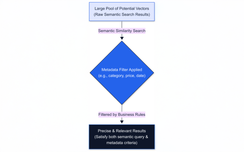
Vector search has transformed how applications retrieve information by using embeddings to find semantically similar content. However, raw similarity often isn't enough in real-world AI applications. This is where metadata filtering becomes crucial – it lets us constrain vector search results based on structured attributes like category, price, user ID, or timestamp.
By combining semantic similarity with filters, we ensure results are not only relevant in meaning but also meet specific business criteria. For example, a user searching for "laptops" might only want models under $1000 – semantic search finds similar products, and a price metadata filter guarantees the results are within budget.
In this comprehensive guide, we'll explore how four popular vector databases – Pinecone, Weaviate, Milvus, and Qdrant – handle metadata filtering. We'll dive into the business impact, common pitfalls, selection criteria, technical implementation details, and emerging trends to help engineering leaders make informed decisions for their AI infrastructure.
Business Impact of Metadata Filtering
Implementing effective metadata filtering can significantly boost the business value of AI-driven search and recommendations:
- Personalized search: By filtering on user attributes, organizations can deliver tailored results – showing content in preferred languages or products available in a user's region. This drives higher engagement and conversion rates.
- Rule-based recommendations: Applying business rules (like in-stock items or items in the user's price range) on top of similarity matches creates more trustworthy recommendations that respect real-world constraints.
- Hybrid search capabilities: Combining semantic vector search with traditional structured filtering or keyword matching enables powerful use cases. For example, an e-commerce search might use a vector query for relevance but also require `category = "electronics"` and `brand = "Apple"`.
- Fine-grained content moderation: Exclude items with certain tags or attributes, ensuring appropriate content delivery.
- Time-bound queries: Limit results to recent documents or time-relevant content.
- Multi-tenant isolation: Restrict search to a specific customer's data, maintaining security and data boundaries.
Robust filtering transforms raw vector similarity into actionable insights that meet business rules and user intent, dramatically increasing search precision and relevance.
Common Pitfalls in Metadata Filtering
While metadata filtering is powerful, organizations often stumble in its implementation. Here are common pitfalls to avoid:
Overfitting to Metadata
Relying too heavily on metadata filters can backfire. Creating very granular filters for every conceivable attribute might lead to over-constraining the search. This can hide potentially relevant results that don't perfectly match all filters and lead developers to encode business logic that might have been better handled by the model or embeddings.
The key is to use filters for clear-cut constraints (e.g., language or access permissions) but not for subjective qualities already captured by embeddings. A slight mismatch in metadata (such as a typo or missing tag) could exclude the best answer. Define a minimal set of critical filters and let vector similarity handle nuanced relevance.
Neglecting Schema Evolution
Metadata schemas tend to evolve as products and use cases grow. A common mistake is not planning for schema updates – such as adding a new metadata field or changing an attribute's format.
Some databases like Weaviate and Milvus use a schema-first approach (through class definitions or collection schemas), but they offer flexibility through features like schema migrations, dynamic fields, and type safety options. While this might seem restrictive, it can provide better data consistency and validation.
Weaviate Schema Evolution:
- Schema changes require explicit updates through the API or client libraries
- Adding new fields is straightforward but requires a migration step
- Example migration process:
1# Adding a new field to an existing collection
2articles = client.collections.get("Article")
3articles.config.add_property(
4    Property(
5        name="new_field",
6        data_type=DataType.TEXT,
7        description="New field description"
8    )
9)
10- Gotchas:
- Cannot remove required fields without data migration
- Changing data types requires careful planning
- Cross-references need to be updated on both sides
- Schema updates are atomic - partial updates can fail
Milvus Schema Evolution:
- Supports both schema-defined and dynamic modes
- In schema-defined mode (using the 2.5 client API):
- Adding or altering fields requires using the alter_collection_field method
- Example:
1# Using MilvusClient from pymilvus
2from pymilvus import MilvusClient
3
4client = MilvusClient(uri="http://localhost:19530")
5
6# Altering a VarChar field's max_length
7client.alter_collection_field(
8    collection_name="my_collection",
9    field_name="varchar_field",
10    field_params={
11        "max_length": 1024
12    }
13)
14
15# Altering an array field's max_capacity
16client.alter_collection_field(
17    collection_name="my_collection",
18    field_name="array_field",
19    field_params={
20        "max_capacity": 64
21    }
22)
23- In dynamic mode:
- Can add JSON fields without schema changes
- Fields are stored in a JSON column
- Note: See the complete example in the "Dynamic Fields in Milvus" section below
- Gotchas:
- Dynamic fields can't be indexed for filtering (unless using specific JSON field indexing)
- Schema changes require collection reload
- Type validation happens at insert time
- Primary field and partition key can't be altered once set
On the other hand, solutions like Pinecone and Qdrant allow semi-structured JSON metadata without an upfront schema, making it more straightforward to add new fields dynamically. The choice between these approaches depends on your specific needs: if you anticipate frequent schema changes, the flexibility of Pinecone or Qdrant might be preferable, but if data consistency and validation are priorities, Weaviate and Milvus's schema-first approach could be more suitable. In either case, it's wise to design your metadata model with future needs in mind to minimize the need for re-indexing or data migration.
Best Practices for Schema Evolution:
- Plan for common schema changes upfront
- Document all schema changes and their impact
- Test migrations with a subset of data first
- Consider data validation requirements
- Monitor performance impact of schema changes
- Have a rollback strategy for failed migrations
- Use dynamic fields sparingly and only for truly variable data
Underestimating Latency Impact
Applying filters can introduce performance overhead if not handled properly. Many teams underestimate how a complex filter or high-cardinality field can slow down queries. For example, filtering by a common attribute might involve checking a large portion of the dataset, increasing query latency.
It's important to understand how your chosen vector database handles filters under the hood. Does it apply the filter before the ANN (Approximate Nearest Neighbor) search to narrow candidates, or after retrieving the top vectors? Each approach has trade-offs for latency and accuracy.
Measure query times with and without filters and monitor the impact. Sometimes adding an index on the metadata or partitioning the data can drastically reduce latency. Don't assume performance will be fine – benchmark it. Tuning index parameters or using caching strategies may be needed to keep latency low when filters are in play.
Filtering at the Wrong Stage (Pre vs. Post Filtering)
A subtle pitfall is how you combine filtering with vector retrieval. There are two basic strategies:
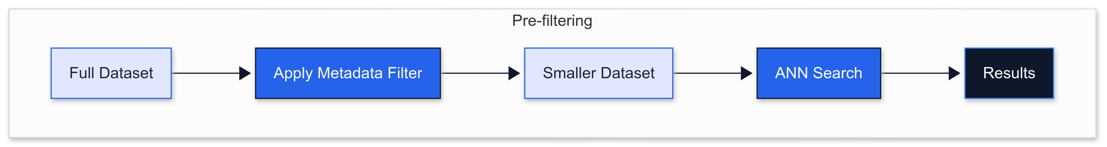
- Pre-filtering: Apply the metadata filter first, then do vector search on the subset. This can speed up queries by searching a smaller set, but if the filter is too restrictive, you risk missing relevant items because the ANN algorithm's graph or tree may be "fragmented" by the filter.
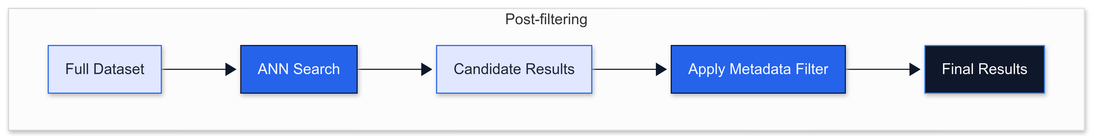
- Post-filtering: Do vector search on the full set, then filter the results. This ensures you don't miss candidates (the vector search sees everything), but you might retrieve many results only to throw most away, wasting computation.
Vector databases handle filtering through various sophisticated mechanisms. Some, like Milvus, use boolean masks that can be efficiently combined with vector search operations. Others, like Qdrant, implement complex filtering systems that can be integrated with vector similarity search, though the specific implementation details vary.
Pinecone offers MongoDB-style query language for metadata filtering, while Weaviate provides GraphQL-based filtering capabilities. The choice of database should consider not just the presence of filtering capabilities, but also how these filters are implemented and their impact on search performance and result quality.
Selecting a Vector Database for Metadata Filtering
How do you choose the right vector database for effective metadata filtering? A clear framework can help evaluate your options:
Filter Expressiveness
Start by mapping your filtering requirements (e.g., numeric ranges, exact match, text contains, geo-location, boolean flags). Different platforms support different operators:
- Weaviate supports GraphQL-based filtering with operators like Equal, NotEqual, Greater/Less Than, text search, array operations, and geo-spatial queries, along with cross-reference filtering capabilities.
- Pinecone supports a MongoDB-inspired query language with equality, inequality, ranges, `$in` arrays, existence checks, and logical AND/OR. For text pattern matching, it uses namespace-based filtering and metadata field type validation.
- Milvus allows boolean expressions with `AND/OR`, supports wildcard `LIKE` for strings, `contains_any` for arrays, and offers hybrid search capabilities with numeric range queries.
- Qdrant supports rich boolean logic (`must`, `should`, `must_not`) with exact match and numeric range conditions, plus geo-spatial filtering and payload-based filtering.
Evaluate which database naturally supports the types of filters you need. If you need complex text pattern matching on metadata, Pinecone (which lacks a `LIKE` operator) might be less suitable than Weaviate or Milvus. If you need nested or hierarchical filters, Qdrant's JSON-based approach could be more appropriate.
Performance and Scale
Consider how each database handles filtering at scale:
- Qdrant allows creating payload indexes on fields to speed up filtering, similar to adding an index in a SQL database. These indexes help evaluate filters faster and inform the query planner about filter selectivity, while supporting distributed deployments.
- Pinecone, as a managed service, abstracts away index tuning but provides namespaces and metadata filtering which they optimize internally, with both serverless and pod-based deployment options.
- Milvus can use bitmap indexes for low-cardinality fields (generally fewer than 500 distinct values) and will perform pre-filtering when possible to reduce search load, while supporting distributed architecture and GPU acceleration. For high-cardinality fields, it uses alternative indexing strategies.
- Weaviate's performance depends on its underlying index configuration, scalar data storage efficiency, and GraphQL query optimization, with support for sharding by class or tenant.
Also consider how they scale out: Pinecone can partition data into pods, Weaviate can be sharded by class or tenant, and both Qdrant and Milvus support distributed deployments. If your dataset is very large or you have strict latency SLAs, you might favor the more mature or optimized engine for filtering.
Ease of Use & Integration
The development experience matters:
- Pinecone offers a simple REST API: you just upsert vectors with metadata JSON, then query with a filter dict, making it ideal for quick prototyping.
- Weaviate uses GraphQL (or client SDKs) which is powerful but has a learning curve, though it provides comprehensive module-based architecture.
- Milvus requires you to define a schema and use its client or API, including writing expressions as strings, but offers good production deployment capabilities.
- Qdrant's filter syntax is JSON-based, which many find intuitive, especially if coming from NoSQL, with good Python integration.
Consider your stack as well: Weaviate's GraphQL might integrate well if you already use GraphQL in your backend. Qdrant and Milvus have robust Python clients which integrate nicely into AI workflows. Pinecone is often used with frameworks like LangChain for quick AI prototyping.
Schema Flexibility
Schema management is a crucial factor:
- Pinecone and Qdrant allow dynamic metadata – you can attach any key-value pairs per vector. This is great for agility but puts the onus on you to enforce consistency.
- Weaviate enforces a schema – all objects of a class have the same fields defined ahead of time, and you must migrate the schema to add new fields. This ensures consistency and can optimize storage but is less flexible.
- Milvus supports both schema-defined and dynamic modes, offering flexibility while maintaining type safety options. The dynamic mode allows JSON-like flexibility while still providing structure through collection definitions.
Think about whether your metadata is well-defined and static (then a strict schema is fine) or evolving/unstructured (in which case a schemaless approach is easier).
Ecosystem and Advanced Features
Consider the broader ecosystem:
- Weaviate has modules for full-text search (BM25), reranking capabilities, and even generative model integration, enabling advanced hybrid search.
- Pinecone has introduced support for sparse-dense vectors, which can be used to achieve hybrid search through both serverless and pod-based deployments. The serverless option provides more flexibility in alpha parameter tuning, while pod-based deployments offer direct hybrid search capabilities.
- Milvus can integrate with third-party search and offers multiple index types, GPU acceleration, and active open-source community support.
- Qdrant focuses on core vector operations but is often integrated into pipelines where an LLM might generate a filter, with good payload-based filtering capabilities.
Community and support are part of this: Pinecone is closed-source but offers enterprise support; Weaviate, Milvus, and Qdrant all have active open-source communities and forums.
Technical Guide: Metadata Filtering Implementation
Let's look at how to implement metadata filtering on each platform, including code snippets.
For hands-on examples and executable code demonstrating the concepts discussed below, please refer to our companion GitHub repository
Pinecone – Filtering by Metadata
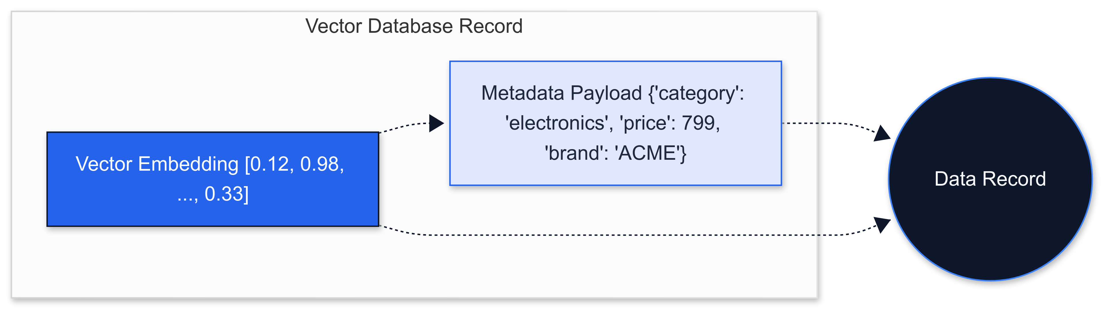
In Pinecone, you attach arbitrary metadata as a JSON dictionary to each vector when upserting. At query time, you provide a `filter` object to restrict results.
1import pinecone
2pinecone.init(api_key="YOUR_API_KEY", environment="us-west1-gcp")
3
4# Assume an index 'products' is already created
5index = pinecone.Index("products")
6
7# Upsert a vector with metadata
8index.upsert([
9    ("prod1", [0.12, 0.98, ... 0.33], {"category": "electronics", "price": 799, "brand": "ACME"})
10])
11
12# Query with a filter
13query_vector = [0.15, 0.95, ... 0.30]
14response = index.query(
15    vector=query_vector,
16    top_k=5,
17    filter={
18        "category": {"$eq": "electronics"},
19        "price": {"$lte": 1000}
20    },
21    include_metadata=True
22)
23
Pinecone implicitly ANDs multiple fields. The result will only contain vectors that satisfy those metadata constraints, sorted by vector similarity score.
Pinecone also has the concept of namespaces – essentially separate sub-indexes – which can be used as a coarse filter (e.g., one namespace per user or per data type).
Important Note on Serverless String Fields: When using Pinecone's serverless indexes, there's a critical limitation with string field filtering. Large string fields that aren't explicitly whitelisted as filterable cannot be used in filters. This can be particularly challenging when working with text-heavy metadata. Here are some practical workarounds:
- Pre-process and Normalize Strings:
1# Instead of storing raw text
2metadata = {
3    "description": "This is a very long product description..."  # Won't be filterable
4}
5
6# Store normalized, shorter versions
7metadata = {
8    "description": "This is a very long product description...",
9    "description_keywords": "product,electronics,new"  # Filterable short string
10}
11
2. Use Enumerated Values:
1# Instead of free-form text
2metadata = {
3    "status": "in_progress_with_multiple_steps"  # Long string
4}
5
6# Use enumerated values
7metadata = {
8    "status": "in_progress"  # Short, predefined value
9}
10
3. Split Long Fields:
1# Instead of one long field
2metadata = {
3    "full_address": "123 Main Street, Suite 456, City, State, ZIP"  # Too long
4}
5
6# Split into filterable components
7metadata = {
8    "street": "123 Main Street",
9    "suite": "456",
10    "city": "City",
11    "state": "State",
12    "zip": "ZIP"
13}
14
4. Use Namespaces for Coarse Filtering:
1# Instead of filtering on long strings
2index.upsert(
3    vectors=[...],
4    namespace="electronics",  # Use namespace for category
5    metadata={"price": 799}  # Keep metadata fields short
6)
7
Sparse-Dense Hybrid Search in Pinecone: Pinecone supports sparse-dense hybrid indexes, which combine traditional vector search with sparse representations (similar to keyword search). This enables hybrid search capabilities that can complement metadata filtering. When using these hybrid indexes, you can adjust the weight between sparse and dense components using an alpha parameter. For serverless indexes, Pinecone recommends using separate dense-only and sparse-only indexes for more flexibility. Only indexes using the dotproduct distance metric support querying sparse-dense vectors.
Best Practices for Serverless String Fields:
- Keep string fields short and focused
- Use enumerated values where possible
- Consider using namespaces for broad categorization
- Pre-process text to extract key information
- Document which fields are filterable in your schema
- Test filter performance with your actual data patterns
- Consider using pod-based indexes if you need extensive string filtering
Weaviate – Filtering with GraphQL Queries
Weaviate organizes data into collections (previously called classes). Filtering is done via a `where` clause in GraphQL queries, or via helper methods in client libraries.
A typical Weaviate query in GraphQL might look like:
1{
2  Get {
3    Article(
4      nearVector: { vector: [0.15, 0.95, ... 0.30], distance: 0.0 },
5      where: {
6        operator: And,
7        operands: [
8          { path: ["category"], operator: Equal, valueText: "electronics" },
9          { path: ["price"], operator: LessThanEqual, valueNumber: 1000 }
10        ]
11      },
12      limit: 5
13    ) {
14      name
15      price
16      category
17      _additional { score }
18    }
19  }
20}
21
Using the Python client (v3): v4 this has changed see the notebooks for reference.
1import weaviate
2from weaviate.classes.config import Property, DataType
3
4client = weaviate.Client("http://localhost:8080")
5
6# Create a collection with properties
7client.collections.create(
8    "Article",
9    properties=[
10        Property(name="title", data_type=DataType.TEXT),
11        Property(name="body", data_type=DataType.TEXT),
12    ]
13)
14
15# Query with filters
16near_vec = {"vector": [0.15, 0.95, ... 0.30]}
17where_filter = {
18    "operator": "And",
19    "operands": [
20        {"path": ["category"], "operator": "Equal", "valueText": "electronics"},
21        {"path": ["price"], "operator": "LessThanEqual", "valueNumber": 1000}
22    ]
23}
24
25result = client.query.get("Article", ["name", "price", "category"])\
26    .with_near_vector(near_vec)\
27    .with_where(where_filter)\
28    .with_limit(5)\
29    .do()
30
Important Notes:
- Collection names must start with an upper case letter (following GraphQL conventions)
- Property names must start with a lower case letter
- Auto-schema is enabled by default but can be disabled for better control
- When adding new properties to an existing collection, you'll need to:- Export existing data- Re-create the collection with the new property- Import the data back
BM25 and Inverted Index Tuning: Weaviate offers sophisticated tuning for its inverted index and BM25 search capabilities, which complements its metadata filtering. You can configure stopwords via the `invertedIndexConfig`, allowing for presets by language (e.g., "en") plus custom additions and removals. As of version 1.18, stopwords are indexed in the inverted index but not in the tokenized query. The BM25 algorithm parameters are also customizable, with two key parameters: `k1` (default: 1.2), which controls term frequency saturation, and `b` (default: 0.75), which controls document length normalization.
Filter Performance Optimization: While Weaviate's default HNSW-flat scalar store works adequately for filtering, version 1.25 introduces significant improvements with inverted-index acceleration. This enhancement dramatically improves query performance when filtering, especially for large datasets. If you're experiencing slow filtering operations with earlier versions, upgrading to take advantage of this optimization path is recommended.
Cross-Reference Filtering: Weaviate's filtering is particularly powerful for its ability to filter on reference properties and geolocation. For example, if `Article` has a reference to a `Category` collection, you could filter articles by category name with a path like `["category", "Category", "name"]`.
Milvus – Scalar Filtering with Boolean Expressions
Milvus uses boolean expressions (SQL-like `WHERE` clauses) in search or query methods. The expression syntax covers standard operations: equality, inequality, comparison, and logical AND/OR.
1from pymilvus import MilvusClient
2
3# Connect to Milvus
4client = MilvusClient(uri="http://localhost:19530")
5
6# Prepare search parameters
7query_embedding = [0.15, 0.95, ... 0.30]
8search_results = client.search(
9    collection_name="Products",
10    data=[query_embedding],
11    limit=5,
12    filter='category == "electronics" && price <= 1000',
13    output_fields=["category", "price"]
14)
15
Dynamic Fields in Milvus:
Milvus 2.5 provides support for dynamic fields through a reserved field named `meta` of JSON type. When enabled, any fields not defined in the schema are automatically stored in this JSON field as key-value pairs:
1from pymilvus import MilvusClient
2
3# Connect to Milvus
4client = MilvusClient(uri="http://localhost:19530")
5
6# Create a collection with dynamic fields enabled
7client.create_collection(
8    collection_name="my_collection",
9    dimension=128,
10    enable_dynamic_field=True  # Enable dynamic fields
11)
12
13# Insert data with dynamic fields
14client.insert(
15    collection_name="my_collection",
16    data=[
17        {
18            "id": 1,
19            "vector": [0.1, 0.2, 0.3, 0.4, 0.5],  # Vector values (must match dimension)
20            "category": "electronics",             # Schema field
21            "color": "red",                        # Dynamic field - stored in $meta
22            "tags": ["premium", "sale"]            # Dynamic field - stored in $meta
23        }
24    ]
25)
26
27# Define a query vector for search
28query_vector = [0.1, 0.2, 0.3, 0.4, 0.5]  # Must match dimension in collection
29
30# Filter using dynamic fields
31results = client.search(
32    collection_name="my_collection",
33    data=[query_vector],
34    limit=5,
35    filter='color == "red"',  # Filtering on dynamic field
36    output_fields=["category", "color", "tags"]
37)
38
Important notes:
- Dynamic fields can be used for filtering just like schema-defined fields
- You can create indexes on dynamic fields for better query performance:
1   client.create_index(
2       collection_name="my_collection",
3       field_name="color",               # Name of the dynamic field to index
4       index_type="INVERTED",            # Index type for the field
5       index_name="color_index",         # Name for the index
6       params={
7           "json_path": "color",         # JSON path to the key
8           "json_cast_type": "varchar"   # Type to cast the value to
9       }
10   )
11- Dynamic fields are particularly useful for:
- Evolving schemas where new attributes may be added frequently
- Sparse data where entities may have different sets of attributes
- Working with semi-structured data from external sources
Enabling BitMap and Inverted Indexes for Filtering: To use the LIKE operator for string pattern matching, you must explicitly enable the wildcard index when creating the collection:
1# Create collection with wildcard index enabled
2schema = CollectionSchema([
3    FieldSchema(name="id", dtype=DataType.INT64, is_primary=True),
4    FieldSchema(name="embedding", dtype=DataType.FLOAT_VECTOR, dim=128),
5    FieldSchema(name="description", dtype=DataType.VARCHAR, max_length=500)
6])
7
8collection = Collection(
9    name="Products",
10    schema=schema,
11    properties={
12        "wildcard": True  # Enable wildcard index for LIKE operations
13    }
14)
15
16# Now you can use LIKE in your queries
17search_params = {
18    "data": [query_embedding],
19    "anns_field": "embedding",
20    "param": {"metric_type": "IP", "params": {"nprobe": 10}},
21    "limit": 5,
22    "expr": 'description LIKE "%electronics%"'  # Wildcard search enabled
23}
24
Important Notes on Data Types:
- FLOAT/DOUBLE Filtering:
- Milvus doesn't support direct filtering on FLOAT/DOUBLE fields
- Common error: `"unsupported data type for filtering: FLOAT"`
- Workaround: Convert to INT64 (e.g., store price in cents)
1   # Store as INT64 (cents) instead of FLOAT
2   metadata = {"price_cents": 9999}  # Filterable
3   expr = 'price_cents <= 10000'  # $100.00
4
2. String Field Limitations:
- Milvus 2.5: Text Match (Inverted Index) offers order of magnitude QPS over Wildcard Match
- BitMap Index: Up to 6.8x performance gain for tag filtering
- LIKE operator requires wildcard index (v2.4+)
- Best practice: Prefer Text Match over LIKE for better performance
3. Type Validation:
- Strict type checking at insert time
- Common error: `"type mismatch: expected INT64, got FLOAT"`
Best Practices for Milvus Filtering:
- Use Text Match over LIKE for better performance
- Enable BitMap Index for low-cardinality fields
- Convert FLOAT/DOUBLE to INT64 for filtering
- Monitor query performance with different filter combinations
- Test type validation with your actual data
- Document your data type conversion strategy
The key part is the `expr` string: `'category == "electronics" && price <= 1000'`. Milvus will interpret this expression and ensure that only entities satisfying it are considered in the search. Internally, Milvus first applies scalar filtering to narrow down the candidates, and then performs the ANN search on that subset.
Milvus also offers a separate `query()` method for pure scalar queries without vector similarity, and supports partitioning data for high-level filtering.
Bitmap Index Limitations: It's important to note that Milvus' bitmap indexes, which can significantly improve query performance for filtered searches, are only available for certain scalar types. According to Milvus documentation, bitmap indexes are specifically designed for low-cardinality fields (generally fewer than 500 distinct values) and are not compatible with floating-point types (FLOAT, DOUBLE) and JSON data types due to their complex structure or binary incompatibility. This limitation should be considered when planning string filtering operations in Milvus.
Best Practices for Milvus Filtering:
- Use Text Match over LIKE for better performance
- Enable BitMap Index for low-cardinality fields
- Convert FLOAT/DOUBLE to INT64 for filtering
- Monitor query performance with different filter combinations
- Test type validation with your actual data
- Document your data type conversion strategy
Milvus 2.5 has significantly improved its developer experience with better documentation and more intuitive APIs. The MilvusClient interface provides a streamlined approach to common operations, while maintaining powerful capabilities for advanced use cases. When implementing complex filtering, the new Text Match capability (offering 400x QPS improvement over Wildcard Match) and BitMap indexes should be considered for optimal performance.
Qdrant – Payload Filtering in JSON
In Qdrant, each vector can have an associated JSON payload. Filtering is done by sending a JSON filter object in your search or query request.
1from qdrant_client import QdrantClient, models
2
3client = QdrantClient(url="http://localhost:6333")
4query_vector = [0.15, 0.95, ... 0.30]
5
6# Construct filter using models
7filter_conditions = models.Filter(
8    must=[
9        models.FieldCondition(
10            key="category", match=models.MatchValue(value="electronics")
11        ),
12        models.FieldCondition(
13            key="price", range=models.Range(lte=1000.0)
14        )
15    ]
16)
17result = client.search(
18    collection_name="Products",
19    query_vector=query_vector,
20    query_filter=filter_conditions,
21    limit=5,
22    with_payload=True
23)
24
Creating and Using Payload Indexes: To optimize filtering performance, you can create payload indexes on specific fields. Here's how to set up and use them:
1# Create a collection with payload indexes
2client.create_collection(
3    collection_name="Products",
4    vectors_config=models.VectorParams(
5        size=128,
6        distance=models.Distance.COSINE
7    ),
8    optimizers_config=models.OptimizersConfigDiff(
9        indexing_threshold=0  # Index immediately
10    )
11)
12
13# Create payload indexes for frequently filtered fields
14client.create_payload_index(
15    collection_name="Products",
16    field_name="category",
17    field_schema=models.PayloadFieldSchema(
18        data_type=models.PayloadFieldType.KEYWORD
19    )
20)
21
22# Create a range index for numeric fields
23client.create_payload_index(
24    collection_name="Products",
25    field_name="price",
26    field_schema=models.PayloadFieldSchema(
27        data_type=models.PayloadFieldType.FLOAT
28    )
29)
30
31# Create a geo index for location-based filtering
32client.create_payload_index(
33    collection_name="Products",
34    field_name="location",
35    field_schema=models.PayloadFieldSchema(
36        data_type=models.PayloadFieldType.GEO
37    )
38)
39
40# Example of using indexed fields in a query
41filter_conditions = models.Filter(
42    must=[
43        models.FieldCondition(
44            key="category",  # Uses keyword index
45            match=models.MatchValue(value="electronics")
46        ),
47        models.FieldCondition(
48            key="price",  # Uses range index
49            range=models.Range(
50                gte=100.0,
51                lte=1000.0
52            )
53        ),
54        models.FieldCondition(
55            key="location",  # Uses geo index
56            geo=models.GeoRadius(
57                center=models.GeoPoint(
58                    lon=13.404954,
59                    lat=52.520008
60                ),
61                radius=1000.0  # meters
62            )
63        )
64    ]
65)
66
Best Practices for Payload Indexes:
- Create indexes only for fields you frequently filter on
- Use appropriate index types:- KEYWORD for exact string matches- INTEGER/FLOAT for numeric ranges- GEO for location-based queries
- Monitor index size and query performance
- Consider the trade-off between index overhead and query speed
- Use composite indexes for frequently combined filters
Common Gotchas:
- Indexes increase storage requirements
- Not all filter operations benefit from indexes
- Indexes are created asynchronously - check status with:
1# Check index creation status
2index_info = client.get_collection(collection_name="Products")
3print(index_info.payload_indexes)
4
Qdrant's JSON-based payload approach provides flexibility similar to document databases while maintaining vector search performance. This makes it particularly suitable for applications with evolving data models or where nested metadata is important for filtering. The ability to add payload indexes incrementally allows for performance optimization without upfront schema design.
Qdrant's filter syntax is quite powerful, supporting logical clauses (must, should, must_not) and nested conditions. For example, if your payload has nested JSON (say a field `specs` with subfields), you can filter within that using a `nested` condition.
Qdrant applies the filter in conjunction with the vector search, using a query planner that can decide to use payload indexes if available, or even perform purely payload-based search if that's cheaper in extreme cases.
Pros and Cons by Platform
Each vector database has its own approach to metadata filtering. The following table provides a quick comparison of their key features:
| Feature | Pinecone | Weaviate | Milvus | Qdrant |
|---|---|---|---|---|
| Filter Syntax | MongoDB-like | GraphQL-based | SQL-like expressions | JSON-based |
| Schema Required | No | Yes | Yes (with JSON flexibility) | No |
| Deployment | Managed | Self-hosted or managed | Self-hosted or managed | Self-hosted or managed |
| String Filtering | Exact match only | Wildcard, regex | Wildcard (with flag in v2.4+) | Token match, no fuzzy |
| Geo Filtering | No | Yes | No | Yes (requires geo_point type) |
| Nested Filtering | Limited | Yes (references) | Limited (JSON fields) | Yes (nested JSON) |
| Scaling | Automatic | Cluster management | Distributed architecture | Cluster (newer) |
| Hybrid Search | Sparse-dense vectors | BM25 + modules | Via integration | Custom scoring |
| Monthly Cost (50K vectors)(illustrative*) | Higher | Medium | Medium | ~$9 (lowest) |
| Best For | Speed to market | Rich filtering | Massive scale | Flexible filtering |
Here's a detailed rundown:
Pinecone
Pros:
- Extremely easy to use (no schema needed; just attach metadata JSON)
- Fully managed service handles scaling and performance optimizations
- Supports a good range of operators for filtering (MongoDB-style selectors)
- Great for multi-tenant use cases using namespaces plus metadata filters
- No infrastructure to manage
Pinecone offers different deployment options with distinct performance characteristics. Serverless indexes provide auto-scaling and cost efficiency for variable workloads but have limitations with string field filtering. Pod-based deployments offer more predictable performance and better support for extensive string filtering, making them suitable for production workloads with consistent query patterns.
Cons:
- Being closed-source, you have less visibility into how filtering is executed
- No support for advanced string queries (no wildcard or regex filters)
- No built-in geo filtering
- Cloud-only, so not an option for on-premises requirements
Weaviate
Pros:
- Rich filtering capabilities (many operators including textual `Like`, geo queries)
- GraphQL interface allows combining vector search with structured conditions elegantly
- Being open-source, you can self-host and inspect how it works
- Has modules for hybrid search, which can complement metadata filtering
- Strong community and documentation, plus a cloud option
When designing schemas in Weaviate, consider granularity tradeoffs. Smaller units (paragraphs vs. chapters) provide more accurate search but require more vectors and memory. Cross-references between collections can represent relationships but add query overhead. Consider denormalizing data where possible for performance-critical applications.
Cons:
- Requires defining and maintaining a schema, adding overhead for changing data models
- GraphQL approach has a learning curve and can be verbose
- Performance with filters might degrade without appropriate indexes
- Scaling Weaviate horizontally requires managing a cluster
Milvus
Pros:
- Excellent performance at scale – built for billion-scale vector search
- Filtering is integrated at a low level, often resulting in efficient query execution
- SQL-like syntax is familiar to many and very precise
- Can partition data for query constraints
- Open-source with enterprise support via Zilliz
Cons:
- Highest operational complexity – running a Milvus cluster involves multiple components
- Requirement to predefine schema means less flexibility for ad-hoc metadata
- Expression syntax is not as flexible as Qdrant's JSON for nested data
- Writing expressions in strings requires careful sanitization
Qdrant
Pros:
- Very flexible JSON-based filtering that handles complex and nested conditions
- No schema required; you can add any payload keys you want
- Filtering performance is generally good and can be improved with indexes
- Developer experience is straightforward with a low learning curve
- Open-source and lightweight to run
Cons:
- Being newer, cluster features are still evolving
- No fuzzy text matching out of the box
- High-cardinality data requires indexing to avoid linear filter checks
- Less battle-tested than Milvus for massive scale
Implementation Considerations by Organization Size
Different organization sizes have varying requirements and constraints:
Startups and Small Teams
Startups prioritize speed of development and iteration. A managed solution like Pinecone can be very attractive – allowing vector search and filtering in minutes without worrying about operations. For zero-budget teams comfortable managing a server, Qdrant is an excellent choice – one engineer can run a Docker container with an intuitive API.
Startups also pivot quickly, so schema flexibility is valuable: Pinecone and Qdrant let you evolve your metadata on the fly. That said, if the core product heavily revolves around search and needs advanced filtering logic from day one, Weaviate's richer capabilities might save development of additional features.
Milvus, with its cluster complexity, is usually not a first choice for a tiny team unless their dataset is already huge or they have specific performance needs.
Mid-Size Tech Teams
Mid-size companies start caring more about cost-efficiency and maintainability. At this stage, cost-performance tradeoffs come into play. Pinecone's convenience might be weighed against monthly bills – if too high, teams might consider moving to an open-source solution hosted on their own cloud instances.
Integration with existing systems becomes important. If the company already has a data lake or warehouse, they might prefer a vector database that can integrate via connectors.
Schema management also becomes crucial – as teams and data grow, keeping track of metadata fields and ensuring consistency is a challenge. Weaviate's explicit schema can be useful as documentation and a single source of truth.
Mid-size teams might implement more complex filter logic (like attribute-based access control or personalization rules) and should ensure the chosen database can express those requirements efficiently.
Enterprise Deployments
Enterprises prioritize scale, reliability, security, and compliance. Multi-region availability, data governance, and integration with enterprise data systems are paramount.
Pinecone's managed service is appealing for its robustness with enterprise features. However, some enterprises require on-premises or private cloud deployments for sensitive data or regulatory reasons, making open-source solutions like Milvus or Weaviate attractive.
Fine-grained access control is often needed in enterprise settings, requiring filters based on complex rules (user groups, roles) possibly at query time.
Latency at scale is critical – an enterprise application might require P95 query latency under 50ms even with filters and millions of vectors. Achieving this may require index tuning, payload indexes, or other optimizations.
Cost is considered at scale too – self-hosting on enterprise Kubernetes infrastructure might be cheaper than managed services for very large vector collections. Many enterprises opt for supported versions with features like encryption and audit logging.
Key Metrics for Success
To ensure your vector search with metadata filtering is delivering value, track these key metrics:
- Query Latency (with and without filters): Measure how long each query takes, especially 95th or 99th percentile latency when filters are applied. Monitor the difference between unfiltered and filtered searches.
- Throughput and Scalability: Can the system handle your required queries per second under load? Throughput tests with various filters should be conducted to ensure the solution scales with user demand.
- Filter Precision/Accuracy: Verify that results actually fall within the expected ranges and match the filter criteria consistently.
- Recall under Constraints: When combining semantic search with filters, ensure high recall within the filtered subset. If there are 100 relevant items that satisfy the filter, does your vector search fetch most of them?
- Filter Usage and Distribution: Track which filters are used most often and how selective they are. This informs optimization priorities.
- System Resource Utilization: Monitor CPU, memory, and possibly GPU usage during filtered searches to ensure resource usage is stable and within your hardware budget.
- User Satisfaction Metrics: Consider click-through rates, conversion rates, or qualitative feedback on relevance. A drop in "zero-result queries" after implementing filters is a sign of success.
When implementing metadata filtering, monitoring is crucial regardless of the platform chosen. Each database offers different tools for understanding query performance: Milvus provides detailed metrics on filter evaluation and ANN search, Weaviate offers insights through its monitoring endpoints, Pinecone provides query analytics, and Qdrant allows for detailed telemetry. Establishing baseline performance metrics and regularly testing with your actual data patterns will ensure optimal configuration.
Emerging Trends
The field of vector search is rapidly evolving:
- LLM-Aware Filtering: LLMs are increasingly being used to interpret user intent into filters. For example, an LLM can parse a query like "Show me recent research papers on quantum computing" and infer that "recent" means a year filter. Vector databases may provide more natural-language interfaces for filtering in the future.
- Hybrid Semantic-Structured Search: We're seeing a convergence of traditional search engines and vector search. Vector databases are incorporating more built-in support for hybrid search capabilities, as seen with Pinecone's sparse-dense vectors (with different implementations for serverless and pod-based deployments), Weaviate's BM25 capabilities, and Milvus's integration with third-party search engines. This blurs the line between vector databases and search engines.
- Metadata as First-Class Citizen in Ranking: An emerging idea is to incorporate metadata into the scoring function, not just for binary filtering. For example, preferring items with certain attributes rather than hard filtering. Look for vector databases to add support for custom scoring functions that incorporate metadata.
- Dynamic Schema and Federated Data: The trend is toward flexibility and integration with external data sources. Future systems might offer hooks to call out to an API or database when applying a filter, enabling up-to-date filtering without reindexing vectors.
- Standardization and Query Languages: With each platform having its own filter syntax, there might be a push toward standardization, perhaps a common Vector Query Language that covers vectors and filters. This would make it easier to move between systems.
- Advanced Index Optimization: Platforms are introducing more sophisticated indexing strategies for metadata, as seen with Milvus' bitmap indexes for low-cardinality fields and Weaviate's BlockMax WAND algorithm for improved BM25 performance. These optimizations help balance the trade-offs between search accuracy, latency, and resource usage.
Conclusion and Next Steps
Metadata filtering is essential for making vector search work in real-world applications. Pinecone, Weaviate, Milvus, and Qdrant all provide mechanisms to filter results by metadata, each with its own strengths.
As actionable next steps, consider:
- Evaluate your needs against the platforms: Create a checklist of must-have filter features and compare which database meets your requirements.
- Design your metadata schema thoughtfully: Keep it lean – only include what you'll actually filter or retrieve. Decide if you need a strict schema or flexibility.
- Implement incrementally and test: Start integrating vector search with metadata filters in a non-critical path and gather metrics.
- Optimize and scale: Once confident, deploy it live and monitor. Address any slow queries by analyzing if filtering is the cause.
- Stay updated on new features: These platforms are adding features frequently. Upgrading to a version with better filtering support could immediately benefit your application.
- Plan for the long term: Design your code with abstractions that make switching databases less painful if needed.
By taking these steps, you'll be well on your way to implementing a robust vector search solution that leverages metadata filtering to its fullest potential.
References
This blog post is based on comprehensive research on vector databases and their metadata filtering capabilities. All information has been sourced from documentation, technical guides, and implementation examples for Pinecone, Weaviate, Milvus, and Qdrant.
- Pinecone Documentation: Understanding Hybrid Search
- Pinecone Blog: Introducing support for sparse-dense embeddings
- Milvus Documentation: BITMAP Index
- Milvus Documentation: Index Scalar Fields
- Weaviate Documentation: Collection Definition - InvertedIndexConfig
- Weaviate Documentation: Keyword Search (BM25)
- Weaviate Release Notes: BlockMax WAND Algorithm
- Milvus Blog: Introducing Milvus 2.5: Full-Text Search and Metadata Filtering
- Qdrant Documentation: Payload Indexing
- Milvus Documentation: Text Match Search
- Milvus Documentation: Advance Data Types
- Pinecone Documentation: Serverless Indexes